data8 final prep

• Understanding of confidence interval
• Some Formulas in SD and SE, CLT
• Histogram vs Bar Chart

How to Identify a Numerical Variable

1. Does it represent a measurement or a count?
   1. Measurement: Continuous - Numerical
2. Mathematical Operations
   1. Mean, Sum, Average - Do they have meaning? Yes - Numerical

Histogram vs BarChart

• *Histogram: (Variable (unit) vs Percent per (unit)) A histogram is specifically designed to show the distribution of a single numerical variable. It divides the range of the numerical data into intervals (bins) and displays the frequency or count of observations falling into each bin. This allows one to see the shape of the data, such as its central tendency, spread, and skewness.

• *Bar chart: (Count vs Category) A bar chart is typically used to display and compare the values of categorical variables or to show discrete numerical values for different categories. While a bar chart can represent counts of numerical data if the data is first grouped, a histogram is more fundamentally suited for displaying the distribution of continuous or discrete numerical data across a range.

• Overlaid: Overlaid is typically for same chart, but you have different distributions(multiple variables) or different categories (races for example).

• Bar charts display one numerical quantity per category. They are often used to display the distributions of categorical variables. Histograms display the distributions of quantitative variables.

• All the bars in a bar chart have the same width, and there is an equal amount of space between consecutive bars. The bars can be in any order because the distribution is categorical. The bars of a histogram are contiguous; the bins are drawn to scale on the number line.

• The lengths (or heights, if the bars are drawn vertically) of the bars in a bar chart are proportional to the count in each category. The heights of bars in a histogram measure densities; the areas of bars in a histogram are proportional to the counts in the bins.

Binning Convention:

• Bins are contiguous (no gaps between them, unless a bin has zero count).
• The left endpoint is included in the bin, and the right endpoint is excluded. For example, a bin [10, 20) includes values that are ≥10 and <20. The value 20 would fall into the next bin, e.g., [20, 30).
• The last bin may include its right endpoint to ensure all data is captured, or this is handled by how the bins are specified.

Vertical Axis of the Histogram:

• often represents density or percent per unit on the horizontal axis.
• The area of each bar in a histogram is proportional to the number (or percentage) of data points in the corresponding bin.
• $\text{height of bar}=\frac{\text{area / percentage of data in this bin}}{\text{width of the bin}}$

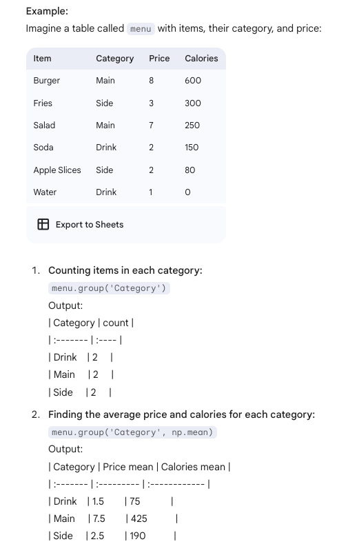
Group vs Pivot Methods

• group method

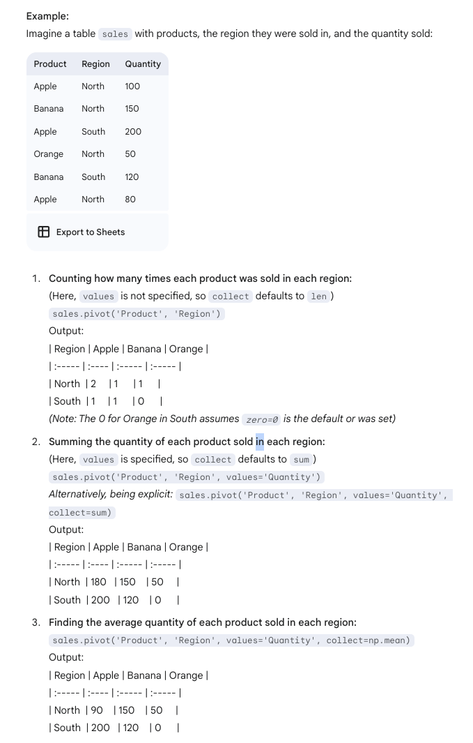
• Pivot Method

The pivot method is used to create a “pivot table” or a contingency table. It allows you to summarize data by cross-tabulating two categorical variables. One variable’s unique values become the new column headers, and the other variable’s unique values become the row labels. The cells of the new table contain aggregated values from a third (optional) column.

Yes, when results are statistically significant, it generally means that the null hypothesis is rejected.

if p value is greater than cutoff, then we fail to reject the null hypothesis.

If p value is less than cutoff, then we reject null, support alternative.

AB Testing / Permutation Test.

What Gets Shuffled:

• To simulate this null hypothesis, you randomly permute (shuffle) the group labels and reassign them to the fixed, observed outcomes.
• Imagine you have all your outcome values written down. Next to each outcome, you have its original group label. In a shuffle:
  • You keep the list of outcome values as is. These are the actual results you observed.
  • You take all the group labels (e.g., if you had 50 in Group A and 50 in Group B, you have fifty ‘A’ labels and fifty ‘B’ labels), put them in a hat (metaphorically), mix them up, and then randomly assign one shuffled label to each of the fixed outcome values.

Confidence Interval

The main purpose is to quantify the uncertainty associated with estimating a population parameter. Since our sample is just one of many possible samples we could have drawn, our sample statistic (e.g., sample mean) is unlikely to be exactly equal to the population parameter. A confidence interval gives us a range of plausible values for that true, unknown parameter.

• We’re 95% confident that the true population parameter lies in this interval.
• We are 95% confident that the method used to generate the interval [A, B] captures the true population mean.” False: There is a 95% probability that the true population parameter lies in this interval. 95% of the time, we would get an Confidence interval that contains the true parameter.

Interpretation (This is CRUCIAL and often a source of pitfalls): A C% confidence level means that if we were to repeat the entire process of sampling from the population and constructing a C% confidence interval many, many times, then we would expect about C% of those constructed intervals to actually contain the true, unknown population parameter.

• For example, if we construct many 95% confidence intervals from different samples from the same population, approximately 95% of these intervals will capture the true population parameter, while about 5% will miss it

What it is NOT:

• It is NOT the probability that a specific, already calculated confidence interval contains the true population parameter. Once an interval is calculated (e.g., [10, 14]), the true parameter is either in it or it’s not. The specific interval doesn’t have a probability associated with containing the fixed parameter; it either does or it doesn’t. The “95%” refers to the success rate of the method in the long run.

Common Pitfalls and Exam-Type Questions

Here are common misunderstandings and ways they might be tested:

1. Misinterpreting the Confidence Level:

   • Pitfall: Saying “There is a 95% probability that the true population mean is between X and Y” for a specific calculated 95% CI [X, Y].
   • Correction: The confidence level applies to the procedure of constructing intervals. For any one specific interval, the true parameter is either in it or not.
   • Exam Question Type:
     • “Which of the following is a correct interpretation of a 95% confidence interval [A, B] for the population mean?”
       • Incorrect option: “The probability that the true population mean is in [A, B] is 0.95.”
       • Correct option (style): “If we were to repeatedly draw samples and construct 95% confidence intervals, about 95% of those intervals would contain the true population mean.” OR “We are 95% confident that the method used to generate the interval [A, B] captures the true population mean.”

2. Relationship Between Confidence Level and Interval Width:

   • Pitfall: Thinking a higher confidence level gives a more precise (narrower) interval.
   • Correction: A higher confidence level (e.g., 99% vs. 95%) requires a wider interval. To be more confident that you’ve captured the true parameter, you need to cast a wider net.
   • Exam Question Type:
     • “If we change the confidence level from 90% to 95%, the width of the resulting confidence interval will: (a) Increase, (b) Decrease, (c) Stay the same, (d) Not enough information.” (Answer: Increase)

3. Relationship Between Sample Size (Original) and Interval Width:

   • Pitfall: Not understanding how sample size affects precision.
   • Correction: A larger original sample size generally leads to a narrower confidence interval (for a fixed confidence level). More data provides a more precise estimate of the population parameter, so the bootstrap distribution of the statistic will typically be less spread out.
   • Exam Question Type:
     • “Researcher A computes a 95% CI from a sample of size 100. Researcher B computes a 95% CI from a sample of size 400 (from the same population). Researcher B’s interval is likely to be [wider/narrower/the same width] as Researcher A’s.” (Answer: Narrower)

4. Relationship Between Data Variability and Interval Width:

   • Pitfall: Forgetting that the inherent variability in the population (and thus the sample) affects the CI width.
   • Correction: Higher variability in the underlying data (larger standard deviation) will lead to a wider confidence interval, as there’s more uncertainty in the estimate. The bootstrap samples will also show more variability.
   • Exam Question Type:
     • “Two different samples of the same size are drawn. Sample 1 has a standard deviation of 5, and Sample 2 has a standard deviation of 10. The 95% CI for the mean from Sample 2 is likely to be [wider/narrower/the same width] than the CI from Sample 1.” (Answer: Wider)

5. What the Interval is For:

   • Pitfall: Thinking the CI is an interval for individual data points or for the sample statistic itself.
   • Correction: A confidence interval is an estimate for an unknown population parameter (e.g., population mean, population proportion). We know our sample statistic (e.g., sample mean) exactly.
   • Exam Question Type:
     • “A 95% CI for the average student height is [65 inches, 68 inches]. Does this mean that 95% of the students in the sample have heights between 65 and 68 inches?” (Answer: No, this is an interval for the population average height, not a description of the spread of individual sample data points.)
     • “True or False: The sample mean always falls within a bootstrap confidence interval for the population mean.” (False. While the bootstrap distribution is centered at the sample mean, the CI is derived from its percentiles. It’s an interval for the population mean.)

6. Bootstrap Mechanics:

   • Pitfall: Forgetting key details like resampling with replacement or that the bootstrap sample size is the same as the original sample size.
   • Correction: Bootstrap samples are drawn with replacement from the original sample and have the same size as the original sample. The bootstrap distribution of a statistic is centered around the value of that statistic in the original sample.
   • Exam Question Type:
     • “Describe one step in generating a bootstrap confidence interval for the median.”
     • “True or False: Bootstrap samples are drawn without replacement from the original sample.” (False)

7. The True Parameter is Fixed:

   • Pitfall: Phrasing interpretations as if the population parameter is variable and has a chance of falling into our specific interval.
   • Correction: The population parameter is a fixed (though unknown) constant. It’s the confidence interval that is variable, changing with each sample.
   • Exam Question Type: (Similar to Pitfall 1, but focuses on the parameter)
     • “A 95% confidence interval is calculated. This means there is a 95% chance that the population parameter will be in this specific interval tomorrow.” (False)

8. “All models are wrong, but some are useful”:

   • Pitfall: Overstating the certainty provided by a CI.
   • Correction: A CI is based on a model (e.g., the bootstrap process assumes the sample is representative). If the sample is biased, the CI will likely be biased too, regardless of the confidence level. The CI quantifies sampling variability, not all sources of error.
   • Exam Question Type:
     • “A survey conducted only via landline phones finds a 95% CI for support for a policy. Can we be 95% confident this interval captures the true support among all adults?” (No, the sampling method introduces bias, which the CI doesn’t account for.)