Decision Tree

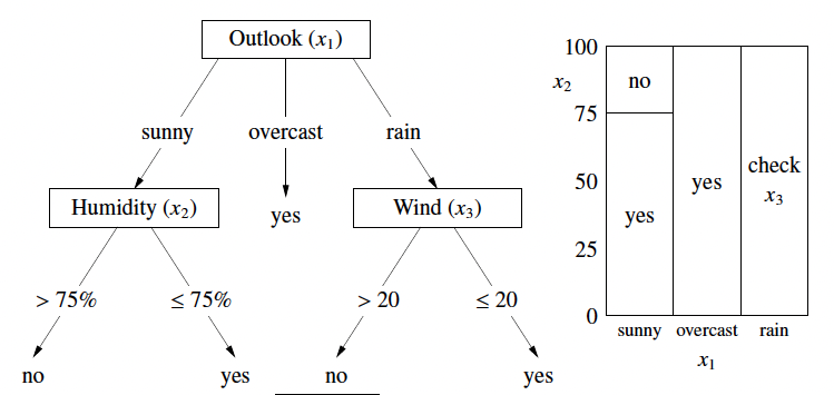
A Decision Tree is a non-linear model used for both classification and regression. A decision tree consists of two types of nodes:

internal nodes: test feature values (usually just one) and branch accordingly. (e.g. is humidity > 75%?)

leaf nodes: specify class $h (x)$ . (e.g. ‘yes’ or ‘no’)

It breaks the input space into rectangular regions using binary decisions.
Interpretable result (inference).
We can think of it as a game of several questions: answering ‘yes/no’ questions to narrow down the answer.
The decision boundary can be arbitrarily complicated.

Warning

Notice how decision trees are selective.

A decision tree will only split features that are useful for making decisions. Therefore, not all features will be used in the final tree.

Why is that? Because at each node, the tree greedily picks the best feature and split value - the one that most reduces the entropy.

✅ Interpretability: The tree tells you which features matter.

✅ Feature Selection: Trees perform implicit feature selection.

⚠️ Instability: Small changes in data can change which features are picked — so decision trees can be unstable (but this is fixed with ensembles like random forests).

🪓 How Trees Learn (Top-Down Recursive Splitting)

Start with all training data S = {1, 2, ..., n}.
At each node:
- If all labels are the same → create a leaf (pure).
- Else:
  - Try all possible splits over all features and all values
  - Choose the split that minimizes the impurity (more on this below)
  - Recur on the left and right subsets.

This is a Greedy Algorithm often known as CART ( Classification and Regression Trees).

🙋‍♂️ How do we choose the best split?

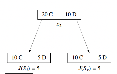
1. ❌ Bad Cost Function: Misclassification Error

Label the majority class C and define the cost J(S) as the # of points not in C.
Problem: Not Sensitive enough. Two splits with very different class balances may have the same cost.

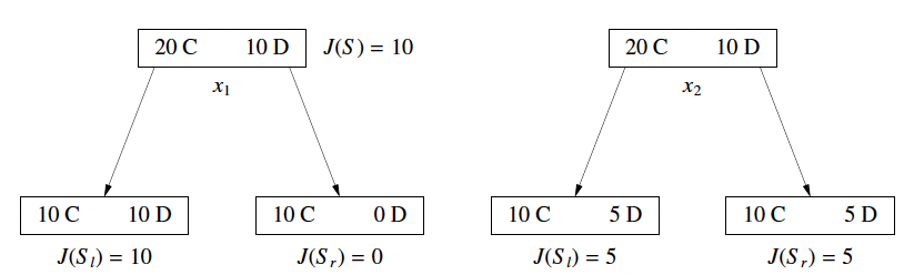
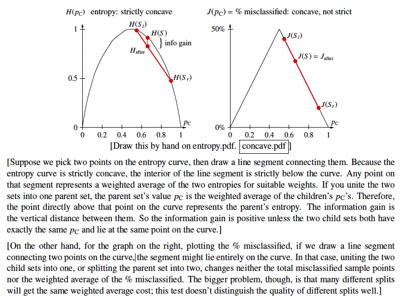
The issue here is cost_before = cost_after = ( $J (S_{l}) + J (S_{r})$ )for both left and right figures even though the left split seems to do a better job.

Weighted Sum of Cost will prefer the right split (which is not a good split).

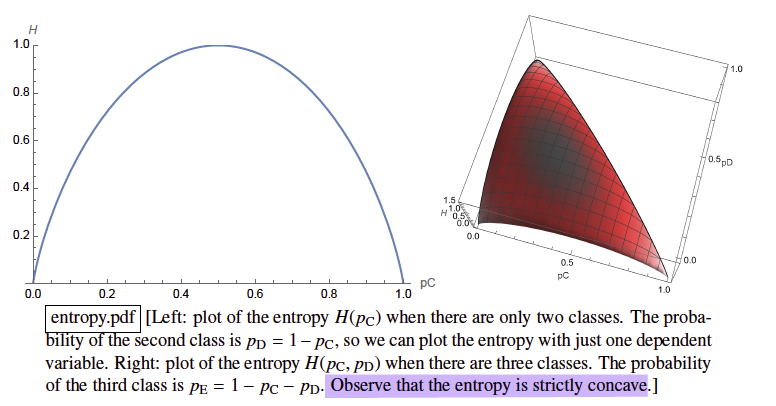
2. ✅ Good Cost Function: Entropy (Information Theory)

Suppose Y be a random class variable and $P (Y = C) = P_{c}$ .

The Surprise of Y being in class C is: $- lo g_{2} P_{c}$ (which is always a positive number)
- event with probability 1 gives us zero surprise.
- event with probability 0 gives us infinity surprise.

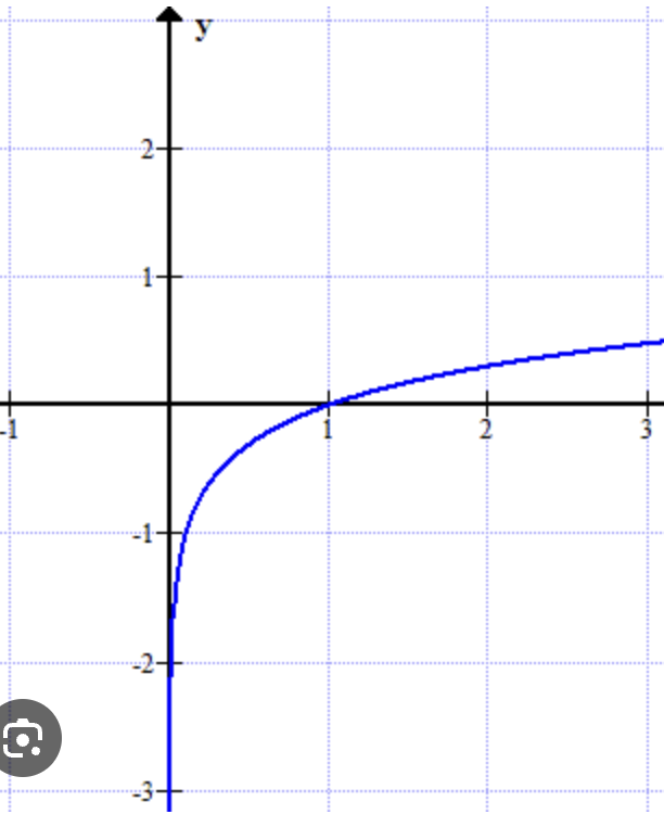
$lo g (x)$ graph. Negative between 0 and 1. $lo g (0) = - \infty$ .

Entropy of an index set S: is the average surprise when you draw a point at random from S.

H (S) = - C \sum P_{c} lo g_{2} P_{c}

If all points belong to one class: $H (S) = - 1 lo g_{2} 1 = 0$
If half of the points in C and the other half in D: $H (S) = - 0.5 lo g_{2} (0.5) - 0.5 lo g_{2} (0.5) = 1$
n points with all different classes: $- lo g_{2} (n) = lo g_{2} (n)$

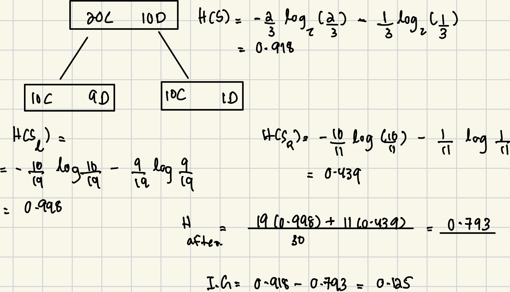
Information Gain

Information gain is defined as:
$H (S) - H_{after}$
where
$H_{after} = \frac{∣ S _{l} ∣ H ( S _{l} ) + ∣ S _{r} ∣ H ( S _{r} )}{∣ S _{l} ∣ + ∣ S _{r} ∣}$

Best Split = Split that maximizes the information gain $H (S) - H_{after}$

> [!danger] Important > > Information gain is always positive except it is `zero` when one child is empty (in which case, it should just be leaf node) or for all C, $P(y_{i} = C | i \in S_{l}) = P(y_{i} = C | i \in S_{r})$}

==Many concave functions work fine as the cost function, including the simple polynomial p(1 − p).==

More Information on Choosing a Split

For binary feature $x_{i}$ , children are $x_{i} = 0 and x_{i} = 1$ .
- $S_{l e f t} = i \in S : x_{i} = 0$
- $S_{r i g h t} = i \in S : x_{i} = 1$
If $x_{i}$ has 3+ discrete values: split depends on application: (multiway splits or binary splits).
If $x_{i}$ is quantitative: sort $x_{i}$ values in S; try splitting between each pair of unequal consecutive values.
If we use radix sort, we can sort in linear time O(n). As we can scan sorted list from left to right, we can update entropy in O(1) time per point.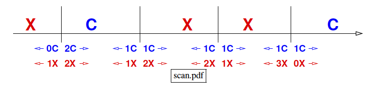

Algorithm and Running Times:

Classification

Walk down tree until leaf. Return its label.
Worst Case Runtime is O(tree depth).
For binary features, tree depth is $\leq$ d. (Quantitative features may go deeper).
Usually (not always) $\leq$ O(logn).

Training

For binary features, try O(d) splits at each node.
For quantitative features, try O(n'd) splits where n’ = points in node. * For each feature, we sort the n' values and try n'-1 thresholds. * Do this for d features → O(n'd) total splits to consider at this node.

Quantitative features are asymptotically just as fast… clever entropy trick”

💡 The clever trick: As you scan from left to right through the sorted feature values, you update the entropy in O(1) time per split.

So the total cost is linear in n′ per feature — no need to recompute from scratch each time.

Each point participate in O(tree depth) nodes, costs O(d) in each node. So for each sample point, it costs O(d * depth).

Thus, running time is O(nd depth)

nd is the size of the matrix X.

Decision Tree Regression

We have explored the decision tree classification in the above paragraphs and now, we will explore regression with decision trees.

Noticeable Differences

Classification trees predict discrete classes.
Regression trees predict real-valued outputs (price, temperature, score, etc.)
Instead of storing the majority class in leaf (as in classification), regression trees store the average of the target values in the leaf.

Decision Tree Regression

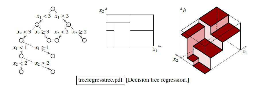
Decision tree creates a piecewise constant regression function.

Leaf stores label $μ_{s} = \frac{1}{∣ S ∣} \sum_{i \in S} y_{i}$
Cost function is the variance of points in subset S: $J (S) = \frac{1}{∣ S ∣} \sum_{i \in S} (y_{i} - μ_{S})^{2}$ .
The cost will be zero if all points in the leaf have the same value.
We choose the split that minimizes the weighted average of the variances of the children after the split.

When should we stop and Why? (Stopping Early)

Why do we stop early?

Limit tree depth for speed
Limit tree size for big data sets
Pure tree may overfit most of the time
Given noise or overlapping distributions, pure leaves tend to overfit; thus, better to stop early and estimate the posterior probabilities.

Cite

When you have strongly overlapping class distributions, refining the tree down to one training point per leaf is absolutely guaranteed to overfit, giving you a classifier akin to the 1-nearest neighbor classifier. It’s better to stop early, then classify each leaf node by taking a vote of its training points; this gives you a classifier akin to a k-nearest neighbor classifier.

Alternatively, you can use the points to estimate a posterior probability for each leaf, and return that. If there are many points in each leaf, the posterior probabilities might be reasonably accurate.

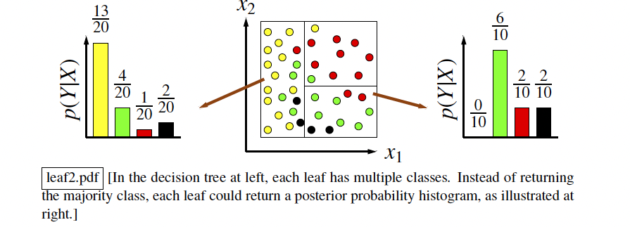
In the case of early stop, the leaves will not be pure, in which case they will return multiple points with:

a majority vote or a posterior probability for Classification problems

an average (mean or median) for Regression problems

So now that we know why stopping early might be a good idea, let’s see HOW we stop early. What are the conditions?

The next split is not doing much (doesn’t reduce entropy / error) enough. (Not the best; can be dangerous; pruning is better).
Most of node’s points (e.g. >90%) have the same class.
Node contains too few points (e.g. < 10 points) for a big data set.
Box’s edges are all tiny (super-fine resolution maybe an overfitting sign).
Depth too deep (not a big problem in general, but bad for speed).
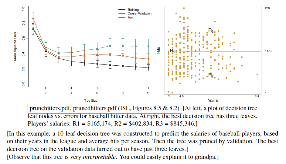
Use validation to compare (best in practice).

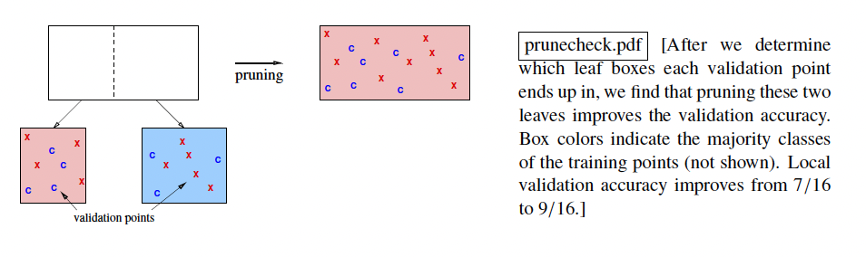
Let’s explore more on the use of validation to decide whether to split the node or not. In general, a better idea is to used a method so called Pruning. Basically, we grow the tree as large as possible and greedily remove splits if the removal of that specific split reduces the validation error.

We do need to do the validation once for each split that we’re considering reversing. This is slow but a rather reliable in practice.

Flow: We split the tree → check validation after the split → try pruning a node → Check validation after the split. If the validation seem to do better after pruning, remove that specific node.

Important Note:

We can only prune the leaves and prune recursively (bottom to top).

The reason why pruning often works better than stopping early is because often a split that doesn’t seem to make much progress is followed by a split that makes a lot of progress. If you stop early, you’ll never find out. Pruning is simple and highly recommended when you have enough time to build and prune the tree.

Number of leaves = Number of Regions.

Validation for each iteration in pruning is not very expensive.

What we can do is compute which leaf each validation point winds up in, and then for each leaf, you make a list of its validation points. So, when we do the validation test for whether to prune the leaf or not, we can just use those points in those two leaves: not an entire validation set.

We have to see how the validation points will be reclassified and how that will change the error rate. In the above figure, pruning results in the leaf labelling as red color. The pruned posterior probability is better than the weighted sum of posterior probabilities of the split children.

Multivariate Splits (Non Axis Aligned Splits)

The idea is that we generate non-axis-aligned splits by other classification algorithms like logistic regression, GDA, SVMs or a random generator. The decision tree then allow these algorithms to find non-linear decision boundaries by making them hierarchical.

By doing so, we may get a better classifier at the cost of worse speed and no-interpretability. Since we’re checking all features at each node (instead of just one feature like in axis-aligned splits), it will slow down the classification.

A good balance is to set a limit on the number of features we check at each tree node.

Ensemble Learning

🪴 Digital Brain

Explorer

Decision Trees

🪓 How Trees Learn (Top-Down Recursive Splitting)

🙋‍♂️ How do we choose the best split?

1. ❌ Bad Cost Function: Misclassification Error

2. ✅ Good Cost Function: Entropy (Information Theory)