Logistic Regression (1958)

Logistic Regression

Despite the name “regression,” logistic regression is mainly used for classification, not regression.

Logistic Regression Function + Logistic Loss Function + Mean Loss Cost Function

• the inputs y’s can be probabilities, can also be 0 or 1 (in most applications).
• usually used for classification
• Fits probabilities in range [0, 1].

In QDA and LDA (generative models) we estimate the underlying data first. In logistic regression, we only care about the posterior probability. (No estimation of the data distribution).

We will use the same X and w as in linear regression. That is we include the fictitious dimension for the bias term $\alpha$.

---

The essence of logistic regression: Find w that minimizes

$$\begin{array}{rl}J& =\sum _{i=1}^{n}L(s(X_i.w),y_i)\\ & =-\sum _{i=1}^n(y_i\ln (s(X_i.w))+(1-y_i)\ln (1-s(X_i.w)))\end{array}$$

The minus term comes from the logistic lost function. We will learn more on this later.

---

Into the Logistic Loss Function

Before we proceed to finding the minimum of the cost function, we should try to understand both the loss function and the cost function. Recall that the logistic loss function is defined as:

$$L(\hat{y},y)=-[y\ln \hat{y}+(1-y)\ln (1-\hat{y})]$$

Important recall: $\ln (x)=-\infty ,x=0$. It does not make sense for us to have a negative infinity loss in general. This is why earlier we said that the loss function must follow — $0<\hat{y}<1$, and $0\le y\le 1$. This aligns with the logistic function a.k.a sigmoid function as the sigmoid function compresses $+\infty ,-\infty$ to approach +1 and -1 respectively but never +1 or -1.

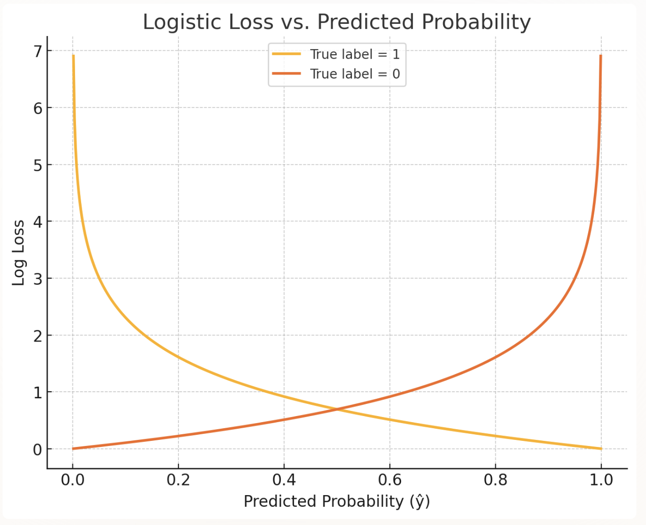
Observation

A good observation here would be to see what the logistic loss is doing intuitively. Evidently, the loss function penalizes harder (larger) if it has a high confident that the label is wrong.

---

Into the Logistic Regression Function

The logistic regression function is defined as:

$$f(w,x,\alpha )=s(w.x+\alpha )\text{where}s(\gamma )=\frac{1}{1+e^{-\gamma }}$$

Now, let’s look at the derivative of the logistic regression function:

$$\begin{array}{rlr}{s}^{\prime }(\gamma )& =\frac{d}{dr}\frac{1}{1+e^{-\gamma }}& \\ & =\frac{e^{-\gamma }}{(1+e^{-\gamma }{)}^2}& =s(\gamma )(1-s(\gamma ))\end{array}$$

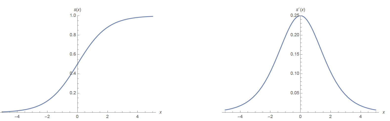Sigmoid and Derivative of Sigmoid

---

Now that we have these information, we can continue our main goal of finding the minimum cost. (i.e $\nabla J_w=0$).

For simplicity of notation, let $s_i=s(X_i\cdot w)$

$$\begin{array}{rl}J& =-\sum _{i=1}^n(y_i\ln (s(X_i.w))+(1-y_i)\ln (1-s(X_i.w)))\\ J& =-\sum _{i=1}^n(y_i\ln (s_i))+(1-y_i)\ln (1-s_i))\\ {\nabla }_{w}J& =-\sum _{i=1}^n\left(y_i.\frac{1}{s_i}.{\nabla }_w{s}_i+(1-y_i).\frac{1}{1-s_i}.{\nabla }_w(1-s_i)\right)\\ {\nabla }_{w}J& =-\sum _{i=1}^n\left(y_i.\frac{1}{s_i}.{\nabla }_w{s}_i-(1-y_i).\frac{1}{1-s_i}.{\nabla }_w(s_i)\right)\\ & =-\sum _{i=1}^n\left(\frac{y_i}{s_i}-\frac{1-y_i}{1-s_i}\right){\nabla }_w{s}_i\end{array}$$

Computation of ${\nabla }_w{s}_i={\nabla }_{w}s(X_i\cdot w)$

$$\begin{array}{rl}{\nabla }_w{s}_i& ={\nabla }_{w}s(X_i\cdot w)\\ & =s_i(1-s_i)\cdot X_i\end{array}$$

So, the previous equation becomes:

$$\begin{array}{rl}{\nabla }_{w}J& =-\sum _{i=1}^n\left(\frac{y_i}{s_i}-\frac{1-y_i}{1-s_i}\right){\nabla }_w{s}_i\\ & =-\sum _{i=1}^n\left(\frac{y_i}{s_i}-\frac{1-y_i}{1-s_i}\right)s_i(1-s_i)\cdot X_i\\ & =-\sum _{i=1}^n(y_i-s_i)X_i\\ {\nabla }_{w}J& =-X^T(y-s)\text{, where }s(Xw)=\left[\begin{array}{c}{s}_1\\ s_2\\ ⋮\\ s_n\end{array}\right]\end{array}$$

The gradient is in d+1 dimension for both logistic regression and linear regression. A sanity check is that you will be subtracting the gradient from the weight vector, so the two must match the dimensions.

Some notes: $X_i$ is a d x 1 column vector. $y_i-s_i$ is a scalar. Transformation to matrix is by sum of linear combinations of $X^T$ columns.

Can we simply set the gradient to zero?

Answer : No. The logistic cost function is non-linear and non-quadratic although it is still convex. Therefore, unlike linear regression, which has a nice quadratic convex bowl, we need to use numerical method like Gradient descent, Newton’s method, etc. to find the global minimum.

---

Using Gradient Descent to find the global minimum.

• The gradient points to the direction of maximum ascent.
• The update rule in gradient descent would be:

$$\begin{array}{rl}w& :=w-ϵ.{\nabla }_{w}J\\ & =w+ϵ(X^T(y-s))\end{array}$$

Generally start w = 0 in practice.

• The update rule in Stochastic gradient descent:

$$\begin{array}{r}w:=w+ϵ(y_i-s(X_i.w)).X_i\end{array}$$

Stochastic gradient descent works best if we shuffle the data beforehand. In cases with large samples, it might converge before we visit all points.

Final Thoughts:

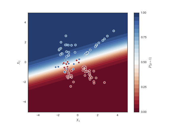
• Logistic regression (classification) gives you a probability that the output is class 1 (true label 1) (assuming binary classification).
• Logistic regression does separate linearly separable points.
• It achieves perfect separation by making the decision boundary infinitely confident—which corresponds to w getting infinitely large.
• w diverges(goes to infinity), but J(w) converges to zero.

---

Newton’s Method

Warning

We assume that the logistic regression cost function (convex, non-quadratic) is guaranteed to converge with Newton’s method.

Taylor's Series

$f(x)=f(a)+f^{\prime }(a)(x-a)+\dots$ Taylor’s Series can be applied to functionsthat are infinitely differentiable (smooth) (including the gradient of logistic regression cost function $\nabla J(w)$

Important Let’s write $\nabla J(w)$ in terms of its Taylor’s Series:

$$\nabla J(w)\approx \nabla J(v)+{\nabla }^{2}J(v)(w-v)+O(\Vert w-v{\Vert }^2)\text{where}{\nabla }^{2}J(v)=\text{Hessian Matrix of J at v}$$

Recall that our main goal is to find the minimum of cost function $J(w)$, which is equivalent to finding $\nabla J(w)=0$.

$$\begin{array}{r}0=\nabla J(v)+{\nabla }^{2}J(v)(w-v)\\ w-v=-\frac{\nabla J(v)}{{\nabla }^{2}J(v)}\\ w=v-\frac{\nabla J(v)}{{\nabla }^{2}J(v)}\\ w=v-({\nabla }^{2}J(v){)}^{-1}\nabla J(v)\end{array}$$

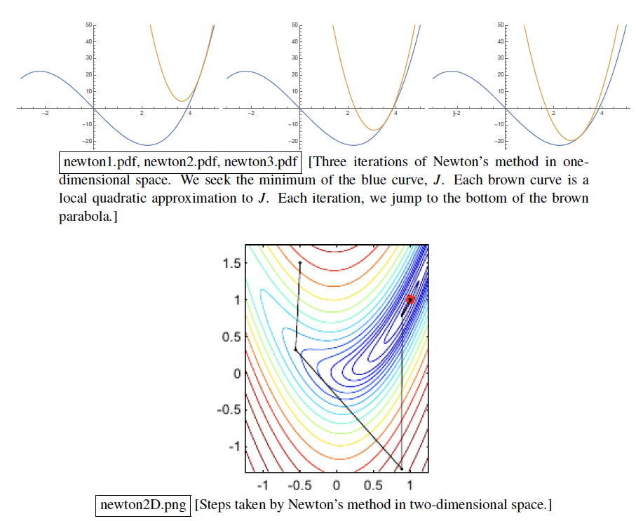
Newton's Method Update Rule

$$w_{t+1}=w_t-({\nabla }^{2}J(w_t){)}^{-1}\nabla J(w_t)$$

Intuitively, we start from a point v, find the gradient and hessian at J(v) = (local quadratic approximation to J). Each iteration, we jump to the bottom of the approximated quadratic function. Next w is the minimum of approximated J that we found from gradient and hessian of real J.

• Also note that this will only work if the Hessian Matrix is invertible. In logistic regression, it does.
• Does not know difference between minima, maxima, saddle points. Logistic regression only has a global minimum.
• If J is quadratic, Newton’s method will converge in one iteration because the approximated (brown graph) is unique. (same first derivative and same second derivative).
• Newton’s method does not work on perceptron risk function, whose Hessian is zero except where Hessian is not even defined.
• Computing Hessian inverse is expensive and need to do it every iteration.
• Only works for smooth function.

---

Deriving Matrix Form for Newton’s method Recall:

$$\text{Update rule: }{w}_{t+1}=w_t-({\nabla }^{2}J(w_t){)}^{-1}\nabla J(w_t)$$ $$\nabla J(w)=-\sum _{i=1}^n(y_i-s_i)x_i=-X^T(y-s)$$ $$s^{\prime }(r)=s(r)(1-s(r))$$

Compute Hessian:

$${\nabla }^{2}J(w)=\sum _{i=1}^n{s}_i(1-s_i)X_i{X}_i^T=X^T\Omega X,\text{where }\Omega =\left[\begin{array}{cccc}{s}_1(1-s_1)& & 0& \\ & \ddots & & \\ 0& & s_n(1-s_n)& \end{array}\right]$$

Important

$\Omega$ is Positive Definite. $X^T\Omega X$ is Positive Semi-Definite. Hessian Matrix PSD implies that J is a convex function.

Pseudocode for Newton’s Method

Important

w $\leftarrow$ 0 Repeat until convergence: $e\leftarrow$ solution to normal equation $(X^T\Omega X)e=X^T(y-s)=-({\nabla }^{2}J(w){)}^{-1}\nabla J(w)$ w $\leftarrow$ w + e

🔺The $\Omega$ here acts in the opposite way as that of from the Weighted Least Squares.

• Misclassified points far from decision boundary - most influence.
• Correct points far from decision boundary - least influence.
• Misclassified points near the decision boundary - medium influence.
• Points (both correct and misclassified) near the decision boundary - medium influence.
• Correct Points near the decision boundary if there is no misclassified points - most influence.

---

LDA vs Logistic Regression

Advantages of LDA:

• For well-separated classes, LDA is more stable compared to Logistic Regression. (Think about the case where the data is linearly separable, but a new ‘outlier’ point can drastically change the decision boundary of the logistic regression).
• For more than two classes, LDA has a natural/more elegant way of handling it. For logistic regression, we will need to use Softmax Regression.
• If the sample is small and normal, LDA is probably more accurate.

Advantages of Logistic Regression:

• More emphasis on the decision boundary.
• If the data is linearly separable (and the data is reliable), linear regression will give a decision boundary that is 100% correct (at least on the training dataset).
• Correctly classified points far from the decision boundary will weigh less. Note that in SVM, these data points have zero effect on the decision boundary. In LDA, all data points are weighted equally.
• Weighting points based on how badly they’re misclassified is good for reducing the Training Error, but it can also be bad if you want a more stable / insensitivity to the data. (if we know the data is bad/ sometimes bad), logistic regression might fail.
• More robust on non-gaussian distribution (eg. large skew distribution).
• Naturally fits labels between 0 and 1.

Danger

• LDA and Logistic Regression has similar decision boundary. i.e. linear decision boundary. But they do not result in the same algorithm.
• QDA and Logistic Regression with quadratic features give quadratic decision boundary but not the same exact classifier.