Regression And Linear Regression

Linear Regression and Logistic Regression are two different decision making algorithms.

Linear Regression:

1. produces a continuous output that can take any real value.

2. Linear Regression Equation:

   $$y={\beta }_0+{\beta }_1{x}_1+\cdots +{\beta }_n{x}_n,y\in \mathbb{R}$$

3. Linear regression uses Mean Squared Error (MSE):

Logistic Regression:

1. produces a probability (between 0 and 1) which is then used for classification.
2. Logistic Regression Equation - uses sigmoid function. $P(y=1)=\frac{1}{1+e^{-\dots }}$ $0\le P(y=1)\le 1$
3. Logistic Regression uses “Log Loss”.

---

In GDA, we were regressing over the posterior probability.

• Choose Form of Regression Function h(x; w) with parameters w. (h = hypothesis)
• Choose a Cost function (objective function) to optimize
  • Usually based on a Loss Function.
    • Empirical Risk (based on the data we have)= Expected Loss (Risk) on data.

Some Regression Functions:

1. Linear: $h(x;w,\alpha )=w.x+\alpha$
2. Polynomial
3. Logistic: $h(x;w,\alpha )=s(w.x+\alpha )$; $s(r)=\frac{1}{1+e^{-}r}$

Some Loss Functions:

Let $\hat{y}$ be the prediction given by $h(x)$; $y$ be the true label.

1. $L(\hat{y},y)=(\hat{y}-y{)}^2$ - squared error - makes it easier to compute.
2. $L(\hat{y},y)=|\hat{y}-y|$ - absolute error - not sensitive to outliers. Harder to optimize.
3. $L(\hat{y},y)=-y\ln \hat{y}-(1-y)\ln (1-\hat{y})$ - Logistic loss, a.k.a cross-entropy. IMPORTANjT* - $y\in [0,1],\hat{y}\in (0,1)$

Observations

• Squared Error is smooth quadratic and convex - meaning it has a closed form solution. Just set gradient = 0 for minimum.
• Logistic Loss is also smooth but non-quadratic and non-linear - meaning the function is still convex (a single global minimum) but need numerical method to find the optimum.

Some Cost functions to Minimize:

1. $J(h)=\frac{1}{n}{\sum }_{i=1}^{n}L(h(x_i),y_i)$ — mean loss (empirical risk). Note that $\frac{1}{n}$ does not matter in optimization.
2. $J(h)=ma{x}_i(L(h(x_i),y_i)$ — if you trust your error. Data is robust.
3. $J(h)={\sum }_{i=1}^n{\omega }_{i}L(h(x_i),y_i)$ — weighted sum.
4. $J(h)=$ cost_1 or cost_2 or cost_3 + $\lambda \Vert w{\Vert }_2^2$ — $l_2$ penalized / regularization.
5. $J(h)=$ cost_1 or cost_2 or cost_3 + $\lambda \Vert w{\Vert }_1$ — $l_1$ penalized / regularization.

Important Notation

• Loss function = a “measure” for each data point.
• Cost function = a “measure” for all data point.

Some famous regression methods:

1. Least Square Linear Regression → Linear Regression Function + Square Error Loss function + Mean Loss.
2. Weighted Least Square Regression
3. Ridge Regression:
4. LASSO:
5. Logistic Regression:
6. Least Absolute Deviations:
7. Chebyshev Criterion:

• 1 to 4 → Quadratic cost: minimize with calculus.
• 4 → Quadratic Program
• 5 → Convex Cost; minimize with gradient descent.
• 6, 7 → Linear Program.

---

[Least Square] Linear Regression (Gauss, 1801)

Linear Regression Function + Squared Loss Function + Cost Function = Mean Loss.

Goal of Least Square Linear Regresssion

Find $w,\alpha$ that minimizes ${\sum }_{i=1}^n(X_i.w+\alpha -y_i{)}^2$. $\alpha$ is a bias term.

X1, X2 are features. The vertical axis is h(x) and y's. h(x) = predicted y (label).

The cost function that we use in linear regression is the sum of squares of errors$(h(x_i)-y_i{)}^2$.

Design Matrix Convention

Design matrix is a nxd matrix of sample points and y is a n vector of scalar labels.

$$\left[\begin{array}{c}-x_1^T-\\ -x_2^T-\\ ⋮\\ -x_n^T-\end{array}\right]$$

where $x_i\in {\mathbb{R}}^d$. The columns are features and the rows are sample points. Typically, n > d if we have enough sample points.

Fictitious Dimension

Rewrite $h(x)=x.w+\alpha$ as

$$\left[\begin{array}{ccc}{x}_{11}& x_{12}& \dots 1\\ x_{21}& x_{22}& \dots 1\\ ⋮& & \end{array}\right]\left[\begin{array}{c}{w}_1\\ w_2\\ ⋮\\ \alpha \end{array}\right]$$

Thus, we will use $X\in {\mathbb{R}}^{n\times (d+1)}$ and $w\in {\mathbb{R}}^{d+1}$. The linear regression problem with bias term can now be rewritten as:

$$argmi{n}_w\Vert Xw-y{\Vert }^2=\text{RSS(w), Residual Sum of Squares}$$

Interpretation: find w that minimizes the squared error

This is a basic Least Squares problem.

$$\begin{array}{rl}\Vert Xw-y{\Vert }^2& =(w^T{X}^T-y^T)(Xw-y)\\ & =w^T{X}^{T}Xw-w^T{X}^{T}y-y^{T}Xw-y^{T}y\\ & =w^T{X}^{T}Xw-2y^{T}Xw-y^{T}y\\ {\nabla }_w\Vert Xw-y{\Vert }^2& =2X^{T}Xw-2X^{T}y\\ 0& =X^{T}X{w}^{\ast }-X^{T}y\\ X^{T}X{w}^{\ast }& =X^{T}y\\ w^{\ast }& =(X^{T}X{)}^{-1}{X}^{T}y\end{array}$$

Note: In this case, there’s always a solution.

• If X has full column rank ⇒ $X^{T}X$ is PD ⇒ (the features are not dependent) ⇒ unique solution.
• Under-constrained ⇒ $X^{T}X$ is PSD ⇒ multiple solutions.
• Over-constrained ⇒ projection (closest in $l_2$ norm solution). (Not in our case because $X{X}^T$ is PSD.)

We use a linear solver to find $w=(X^{T}X{)}^{-1}{X}^{T}y$.

If $(X^{T}X{)}^{-1}$ exists → X is full-column rank → pseudoinverse of X = $X^{{}^{†}}$ = $(X^{T}X{)}^{-1}{X}^T$.

Discussion 6 CS 189 for more.

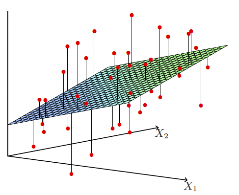
Now, let’s go back to the original problem of predicting the y values. Suppose we have already calculated the weights w, then the projected y values onto the hyperplane with minimum squared error will be:

$$\begin{array}{rl}\hat{y}& =Xw,\text{where}w=(X^{T}X{)}^{-1}{X}^{T}y\\ \hat{y}& =X(X^{T}X{)}^{-1}{X}^{T}y\\ \hat{y}& =X{X}^{†}y\end{array}$$

$X{X}^{{}^{†}}$ is also known as H (the hat matrix) since it puts the hat on the y. If you look carefully, you can also see that this is also just a projection of data onto the column space of X.

If $H=I$, there is no training error since it means all the training points lie on a hyperplane.

Advantages of Linear Regression

• Easy to compute; linear system.
• Unique, Stable Solution unless the system is underconstrained.

Disadvantages of Linear Regression

• Very sensitive to outliers. (because of square errors).
• Fails if $X^{T}X$ is singular but easily fixable.

---

Least Squares Polynomial Regression

Kernel Trick

The idea here is to life the dataset into higher dimensions so that we could do some regression algorithm on the lifted dataset with linear decision boundary. Lifting data into higher dimensions makes it easier to separate (or fit) with a linear model because, in the original space, the relationship is non-linear.

Replace each $x_i$ with $\varphi (x_i)$ with all terms of degree $0\dots p$

Example: $\varphi (x_i)=[x_{i_1}^2+x_{i_1}{x}_{i_2}+x_{i_2}^2+x_{i_1}+x_{i_2}+1$]

But, we need to be cautious since it is very easy to overfit. (too many parameters). A large amount of data can tame the high degree polynomials oscillation. Extrapolation is harder than interpolation.

---

Weighted Least Squares Regression

Linear Regression Function + Squared Loss Function + Weighted Cost Function.

Assign each sample points a weight $w_i$ (this comes from domain knowledge). Greater $w_i$ means focus more on the same i to minimize $({\hat{y}}_i-y_i{)}^2$.

Weighted Least Squares can be formulated as:

$$\begin{array}{rl}& =argmi{n}_w(Xw-y{)}^T\Omega (Xw-y)\\ & \\ & =argmi{n}_w\sum _{i=1}^n{\omega }_i(X_i.w-y_i{)}^2\\ w^{\ast }& =(X^T\Omega X{)}^{-1}{X}^T\Omega y\end{array}$$

Normal Equations / Solve by finding the gradient (the same).

---

Logistic Regression (1958)