Decision Theory

machine-learning cs189

Risk Minimization = Deriving the optimal classifier (r*) Probabilistic Classifier - r Risk - R Risk(r) = Expected loss over all values of x and y for the specific classifier `r Bayes decision rule = Bayes classifier = optimal probabilistic classifier

Posterior Probability Prior Probability

Decision Rule is called a classifier and is denoted by r. Formaljly, $r:{\mathbb{R}}^d\to \pm 1$ Risk is denoted in capital R and is defined as the expected loss over all values of x and y

Continuous Distribution

---

Loss Function

Loss function is generally in the form of $\mathbb{L}(\hat{y},y)$, where $\hat{y}$ is the predicted value by the classifier and y is the truth. Loss Function Value is always $\ge 0$.

Risk Function

Risk is the expected loss over all values of x and y. Note that this is just a scalar value. Formally:

$R(r)=\mathbb{E}[\mathbb{L}(r(X),Y)]$ $={\sum }_x(\left(\mathbb{L}(r(x),1)\cdot P(Y=1|X=x)+\mathbb{L}(r(x),-1)\cdot P(Y=-1|X=x)\right)\cdot P(X=x))$

Rewriting this equation as parameterized by the input would be:

$={\sum }_x\left(\right(\mathbb{L}(r(x),1)\cdot \frac{P(X=x|Y=1)P(Y=1)}{P(X=x)}+\mathbb{L}(r(x),-1)\cdot \frac{P(X=x|Y=-1)P(Y=-1)}{P(X=x)})P(X=x))$

Thus, $=P(Y=1){\sum }_x\mathbb{L}(r(x),1)\cdot P(X=x|Y=1)+P(Y=-1){\sum }_x\mathbb{L}(r(x),-1)\cdot P(X=x|Y=-1)$

Now that we know how to find the Risk, let’s explore the classifier called Bayes Decision, Bayes Classifier that minimizes this risk R(r). Assuming that $\mathbb{L}(1,1)=\mathbb{L}(-1,-1)=0$, (which must hold true for all valid Loss functions): The Optimal Classifier is defined as:

$$r^{\ast }(x)=\{\begin{array}{ll}1,& \text{if }\mathbb{L}(-1,1)\cdot P(Y=1|X=x)>\mathbb{L}(1,-1)\cdot P(Y=-1|X=x)\\ -1,& \text{otherwise }\end{array}$$

🔴 Note that LOSS FN x Probability = Expected Loss

So, we can interpret this as

The optimal classifer is one such that:
	if the LOSS FN is symmetric:
		pick the class with higher posterior probability
	else:
		weight the loss function value before the comparision

---

Example

Suppose 10% of population has cancer, 90% doesn’t.

P(Y = 1) = 0.1 P(Y = -1) = 0.9

The table below is so called likelihood, the probability of the observed evidence given a parameter value. This table is the probability distributions for occupation conditioned on cancer $P(X|Y)$.

job (X)	Miner	Farmer	Other
Cancer (Y = 1)	20%	50%	30%
No Cancer (Y = -1)	1%	10%	89%

We want to calculate that - given a random person whom we only know their occupation, what is the chances that this person has cancer.

Everything above are a mixture of Posterior Probability and Prior Probability. Therefore, we calculate the posterior probability before anything.

$P(X)=P(X|Y=1)P(Y=1)+P(X|Y=-1)P(Y=-1)$ Therefore, we calculate the evidence: P(X)

$P(X=\text{Miner})=0.2\ast 0.1+0.01\ast 0.9=0.029$ $P(X=\text{farmer})=0.5\ast 0.1+0.1\ast 0.9=0.14$ $P(X=\text{other})=0.3\ast 0.1+0.89\ast 0.9=0.83$

Now that we have the evidence, we can calculate the posterior probability: $P(Y=1|X=farmer)=\frac{P(X=\text{farmer}|Y=1)P(Y)}{P(X=\text{farmer})}=\frac{0.5\ast 0.1}{0.14}=0.36$

$P(Y=-1|X=farmer)=1-0.36=0.64$

---

$P(Y=1|X=\text{miner})=0.69$ $P(Y=-1|X=\text{miner})=0.31$

---

$P(Y=1|X=\text{other})=0.036$ $P(Y=-1|X=\text{miner})=0.964$

---

Let’s define a LOSS FUNCTION for this example such that the false negative is considered worse than a false positive. Therefore,

$$\mathbb{L}(\hat{y},y)=\{\begin{array}{ll}5,& \text{if }\hat{y}=-1,y=1\\ 1,& \text{if }\hat{y}=1,y=-1\end{array}$$

Recall our Optimal Bayes Classifier:

$$r^{\ast }(x)=\{\begin{array}{ll}1,& \text{if }\mathbb{L}(-1,1)\cdot P(Y=1|X=x)>\mathbb{L}(1,-1)\cdot P(Y=-1|X=x)\\ -1,& \text{otherwise }\end{array}$$

If the stranger is Farmer for example, x = farmer

$\text{Expected Loss for classifying no cancer:}\mathbb{L}(-1,1)\cdot P(Y=1|X=\text{farmer})=5\ast 0.36=1.8$ $\text{Expected Loss for classifying has cancer:}\mathbb{L}(1,-1)\cdot P(Y=-1|X=\text{farmer})=1\ast 0.64=0.64$ $1.8>0.64$. Therefore, $r^{\ast }(x)=1,\text{for x = farmer}$. Meaning the most optimized classifier will classify that every farmer has cancer.

🟡 However, remember that we have derived this equation so that we will need to do less computation. ^197f68 More specifically, we can calculate the Risk Value by only using the inputs: $P(Y),P(X|Y)\text{and}\mathbb{L}(\hat{y},y).$

Expected Loss for classifying Miner has NO Cancer: $=P(Y=1)\cdot L(-1,1)\cdot P(X=\text{miner}|Y=1)=0.1\ast 5\ast 0.2=0.1$ Expected Loss for classifying Miner has Cancer:

$=P(Y=-1)\cdot L(1,-1)\cdot P(X=\text{miner}|Y=-1)=0.9\ast 1\ast 0.01=0.009$

🔺 Main concept to understand $\to$ Expected Loss for classifying Miner has NO Cancer > Expected Loss for classifying Miner has Cancer. So, a natural way to minimize the loss is to classify that every miner has cancer.

🔺An easier way to see this is, choose the truth value of Loss function of higher expected loss.

Loss Function $\underline{\mathbb{L}(1,-1)}$: Classifier’s loss for choosing 1 while the truth is -1

Bayes Classifier in simple words:

Suppose we have class 1 and class -1. If the expected loss for choosing -1 is higher than that of choosing 1, then the optimal solution is to choose class 1

---

Finishing up the example:

Expected Loss for classifying “Other” has Cancer:

$=P(Y=-1)\cdot \mathbb{L}(1,-1)\cdot P(X=\text{other}|Y=-1)=0.9\ast 1\ast 0.89=0.801$ Expected Loss for classifying “Other” don’t have Cancer: $=P(Y=1)\cdot \mathbb{L}(-1,1)\cdot P(X=\text{other}|Y=1)=0.1\ast 5\ast 0.3=0.15$ Thus, $r^{\ast }(x)=-1\text{for x = other}$

Let’s also calculate the optimal Risk (Bayes Risk)

$R(r^{\ast })=(0.9\ast 1\ast 0.01)+(0.9\ast 1\ast 0.1)+(0.1\ast 5\ast 0.3)=0.249$

🔺 No decision rule gives a lower risk. Bayes risk is the lower bound.

🟩 Conclusion: $r^{\ast }(x=\text{Miner})=1$ $r^{\ast }(x=\text{Farmer})=1$ $r^{\ast }(x=\text{Other})=-1$ Bayes Risk, R(r*) = 0.249 (Bayes Risk represents the minimum probability of the classifier getting it wrong overall)

---

Bayes Classifier for Continuous Distribution

Now that we understand the Bayes Classifier in Discrete Probability, we can now move to the continuous distributions.

Suppose $f_{X|Y=1}(x)$ is the probability distribution of alcohol consumption given that the subject has cancer. So, naturally, $f_{X|Y=-1}(x)$ means the probability distribution of alcohol consumption given that the subject does not have cancer.

We want to make a classifier that can classify whether the person has cancer or not based on the amount of alcohol consumption.

Also suppose we know that our prior probability are $P(Y=1)=\frac{1}{3}$ and $P(Y=-1)=\frac{2}{3}$.

Before we start, let’s define some definition first for the continuous distribution probability.

Risk of classifier “r” R(r) is defined as the expected loss over all x and y.

$R(r)=\mathbb{E}[\mathbb{L}(r(x),Y)]$ Parameterized with inputs: Prior probability, Likelihood and Loss Function $R(r)=P(Y=1)\int \mathbb{L}(r(x),1)\cdot f_{X|Y=1}dx+P(Y=-1)\int \mathbb{L}(r(x),-1)\cdot f_{X|Y=-1}dx$

Note: The first term basically means expected loss for choosing class -1 and the second term is the expected loss for choosing class 1.

Thus, a Bayes Classifier will be:

$$r^{\ast }(x)=\{\begin{array}{ll}1,& \text{if }\int \mathbb{L}(-1,1)\cdot f_{Y=1|X=x}(x)dx>\int \mathbb{L}(1,-1)\cdot f_{Y=-1|X=x}(x)dx\\ -1,& \text{otherwise }\end{array}$$

If we have a symmetric loss function, 0-1 Loss function, the decision boundary / the classifier can be simplified to:

$$r^{\ast }(x)=\{\begin{array}{ll}1,& \text{if }\int f_{Y=1|X=x}(x)dx>\frac{1}{2}\\ -1,& \text{otherwise }\end{array}$$

$0.5=\frac{1}{2}\text{is called the isovalue}$

This simplification is due to the fact that

$P(Y=1|X=x)+P(Y=-1|X=x)=1$ The Optimal Risk / Bayes Risk is

$R(r^{\ast })=min(\int \mathbb{L}(-1,1)\cdot f_{Y=1|X=x}(x)dx,\int \mathbb{L}(1,-1)\cdot f_{Y=-1|X=x}(x)dx)$

---

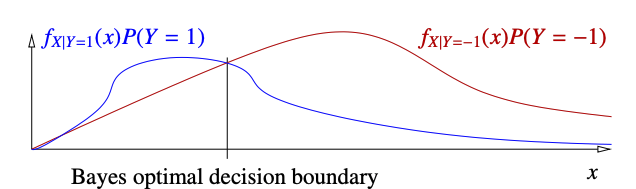
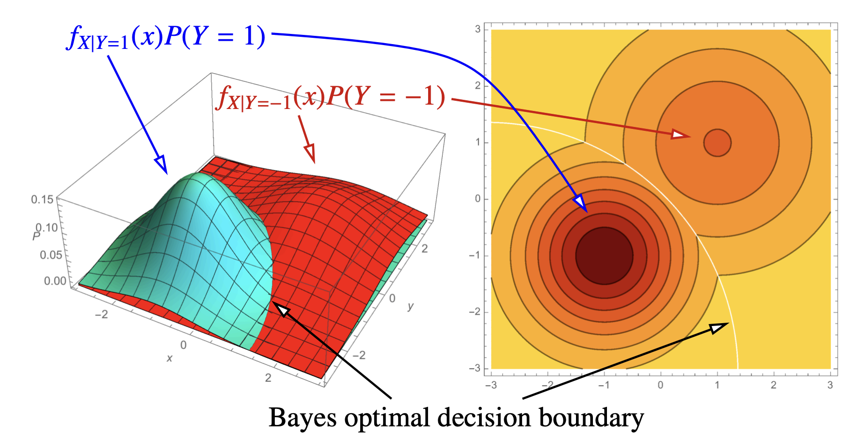
The good part - Looking at the distribution graphically. ( a lot easier )

Figure 3: (Almost) Posterior Continuous Distribution

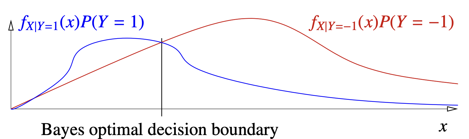
Decision Boundary: $\{x:P(Y=1|X=x)=0.5\}$

In the above picture, we’re assuming that we have a 0-1 LOSS Function. Therefore, naturally, we can choose the one with higher posterior probability to reduce our risk. Recall that $f_{(Y=1|X=x)}=\frac{f_{(X=x|Y=1)}\cdot f_{(Y=1)}}{f_{(X=x)}}$ This is similar to what the curves represent in the given picture except the denominator. But our goal is to compare the two posterior probabilities and thus we can just compare the given function directly without computing the Evidence $P(X)\text{or}{f}_{(X=x)}$

In the case of asymmetrical loss function, we can just scale the curves vertically in the figure above.

The intersecting section between the two curves is the decision boundary illustrated by a line.

Bayes Risk or Optimal Risk : the area under the minimum of functions given.

[[Building Classifiers]]