Building Classifiers

Preface

I will start this note with not much understanding of the models, but by the end of the note, I will revise the different models again, hopefully - with a better understanding of the concept.

3 Ways to Build Classifiers

1. Generative Models (Linear Discriminant Analysis)

Core Idea: Try to learn the underlying probability distributions that generate the data for each class separately. Similar to figuring out how “each class” creates its data points.

2. Discriminative Models (Logistic Regression)

This model Directly Learn the Decision Boundary between classes or the conditional probability $P(Y|X)$ without explicitly modeling the individual class distributions. “The Focus is on Finding WHAT separates the classes from each other .”

3. Find Decision Boundary (Support Vector Machine)

No explicit calculations of Probabilities. Directly find the Optimal Decision Boundary that separates the classes.

⭕ Come back to recognize the advantages and disadvantages of different models.

---

Gaussian Discriminant Analysis

Caution: Although the name is called Gaussian “Discriminant” Analysis, please note that this model is a generative model. The key factor is “How it Learns”. The overall technique is:

• Assume Gaussian Distributions for each class.
• Estimate the parameters (mean and covariance) of these distributions. (Maximum Likelihood Estimation)
• Use Bayes’ theorem to get $P(Y|X)$, the probability of the class given features.

First modeling the probability distribution of each class separately. And learns $P(X|Y)$ The probability of observing features given a class (Hallmark of a generative model). Model $P(X|Y)\to P(Y|X)$.

Fundamental Assumption: Each class has a Normal Gaussian Distribution.

$$X\sim \mathbb{N}(u,{\sigma }^2)$$ $$f(x)=\frac{1}{(\sqrt{2\pi }\sigma {)}^d}\cdot \exp \left(-\frac{\Vert x-\mu {\Vert }^2}{2{\sigma }^2}\right)$$

$\mu ,\sigma \text{and}\text{x are scalars and d = dimension}$

How did we get here?

How did we get this Multivariate Gaussian Distribution with a scalar ${\sigma }^2$ instead of a covariance matrix $\Sigma$?

For each class C, SUPPOSE we know ${\mu }_C$ and variance ${\sigma }_C^2$ which gives us the PDF $f_{X|Y=C}(x)$ and we know prior probability ${\pi }_C=P(Y=C)$.

🚨 In this example, we are assuming that the variance is a scalar, which results in circular iso-contours and not ellipses. This is called isotropic normal distribution because the variance is the same in all directions. Anisotropic Gaussians = isosurfaces are ellipsoids. Also, the Bayes Decision boundary is an ellipse.

From Decision Theory, we know that the optimal classifier $r^{\ast }(x)$ should pick the particular class C such that it maximizes the expected loss : $f_{(X|Y=C)}(x).{\pi }_{Y=C}$

Since we’re considering 0-1 Loss Function, we can also recall the main principle : Pick the class with the highest Posterior Probability

For the sake of simplifying the Math - Maximizing $Q_c(x)=\ln \left((\sqrt{2\pi }{)}^d{f}_{(X|Y=C)}(x).{\pi }_{Y=C}\right)$ is the same as maximizing $f_{(X|Y=C)}(x).{\pi }_{Y=C}$. The term $(\sqrt{2\pi }{)}^d$ is just to cancel out the term in the Gaussian Distribution ^f1b0fd.

Therefore,

$$Q_c(x)=-\frac{{\Vert x-{\mu }_C\Vert }^2}{2{\sigma }_C^2}-d\ln \sigma +\ln {\pi }_C$$

🔺 Notice that $Q_c(x)$ is a quadratic function.

In a 2-class problem, we can also add asymmetric loss function by adding $ln\mathbb{L}(\text{not C},C)$. In a multi-class though, it will be more harder to account for the loss function.

---

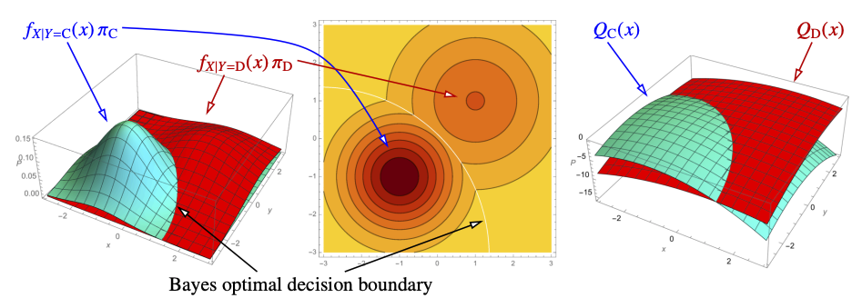
Quadratic Discriminant Analysis (QDA)

Suppose we only have two classes C and D. Then, by Bayes Theorem:

$$r^{\ast }(x)=\{\begin{array}{ll}C,& \text{if }{Q}_C(x)-Q_D(x)>0\\ D,& \text{otherwise }\end{array}$$

Bayes Deicions Boundary is where x satisfies $Q_C(x)-Q_D(x)=0$

$Q_C(x)-Q_D(x)=0$ is a quadratic function and therefore, in 1-dimension, the BDB may have 1 or 2 points. In d-dimension, the BDB is a quadric

🔴 Q: What about the probability that our prediction is correct? This is basically the same as $P(Y=C|X)$

$$P(Y=C|X)=\frac{f_{X|Y=C}.{\pi }_C}{f_X}$$

By the law of total probability:

$$P(Y=C|X)=\frac{f_{X|Y=C}.{\pi }_C}{f_{X|Y=C}.{\pi }_C+f_{X|Y=D}.{\pi }_D}$$

Substitute equation ^25d885,

$$P(Y=C|X)=\frac{e^{Q_C(x)}}{e^{Q_D(x)}+e^{Q_D(x)}}$$ $$P(Y=C|X)=\frac{1}{1+\frac{e^{Q_D(x)}}{e^{Q_C(x)}}}$$ $$P(Y=C|X)=\frac{1}{1+e^{Q_D(x)-Q_C(x)}}$$

Definition

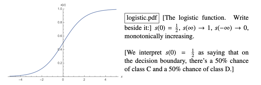
Logistic Function / Sigmoid Function (Real-valued input $\to$ Probability) is in the form of :

$$s(\gamma )=\frac{1}{1+e^{-r}}$$

Putting our probability equation into sigmoid function (monotonically increasing) form:

$$s(Q_C(x)-Q_D(x))=\frac{1}{1+e^{Q_D(x)-Q_C(x)}}$$

🔴 Answer: Now, we can calculate our correctness of the prediction using the sigmoid function.

$\to$ Recall the decision function is $Q_C(x)-Q_D(x)$. The output of the sigmoid function can be interpreted as the probability of the data point belonging to the correct class.

Multi-Class Quadratic Discriminant Analysis (QDA) is quite natural. “multiple decision boundaries that adjoin each other at joints.” The way we do this is by calculating $Q(x)$ of each class and choose the maximum.

Multi-Class QDA partitioning the Feature Space into Regions.

Notice the variance and the boundary

• The dots are the means of each class, and the variances are the circular shapes in the graph. The circular shapes are not spread out equally across different classes, which means that they have different variances.
• Also notice that the decision boundary are not linear since our $Q(x)$ are quadratic functions. come back for updates! Ed Thread

---

Linear Discriminant Analysis (LDA)

Now that we know QDA, let’s explore what happens IF all the Gaussians have the same variance ${\sigma }^2$.

QDA allows each class to have its own covariance matrix ${\Sigma }_k$ where k is a class. LDA is a variant of QDA with Linear Decision Boundaries, where all classes have same covariance matrix ${\Sigma }_k=\Sigma ,\forall k$.

LDA is also less likely to overfit since we assume the same covariance matrix (variance) for all class, reducing the number of parameters to estimate.

Recall that we defined Q(x) to be a natural log of the Gaussian PDF: ^25d885

$$Q_C(x)=-\frac{\Vert x-{\mu }_C{\Vert }^2}{2{\sigma }_C^2}-d\ln {\sigma }_C+\ln {\pi }_C$$

But, we had made an important assumption in LDA that all $\sigma$ are the same. Therefore, the decision boundary $Q_C(x)-Q_D(x)$ is simplified to:

$$Q_C(x)-Q_D(x)=\underset{w\cdot x}{\underbrace{\frac{({\mu }_C-{\mu }_D)\cdot x}{{\sigma }^2}}}-\underset{+\alpha }{\underbrace{\frac{\Vert {\mu }_c{\Vert }^2-\Vert {\mu }_D{\Vert }^2}{2{\sigma }^2}+\ln {\pi }_C-\ln {\pi }_D}}$$

Now, the decision boundary equation is evidently in the familiar linear form of $w.x+\alpha$ as the quadratic terms in $Q_C$ and $Q_D$ cancel out each other.

Similar to what we did in QDA, we can find the correctness probability of our prediction (a.k.a) the posterior probability in the case of 0-1 Loss Function.

$$P(Y=C|X=x)=\frac{1}{1+e^{Q_D(x)-Q_C(x)}}$$ $$P(Y=C|X=x)=\mathbf{s}(Q_C(x)-Q_D(x))$$

To emphasize the linearity, we can rewrite this as:

$$P(Y=C|X=x)=\mathbf{s}(w.x+\alpha )$$

Two Gaussians (red) and the logistic function (black)

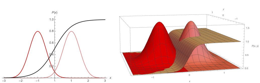
If $Q_C(x)$ is the right Gaussian, the logistic (sigmoid) function is the right Gaussian divided by the sum of two Gaussians. 🔺 Another observation is that the logistic function look 1D even though the Gaussians are 2D. In Higher Dimensions, the logistic function is essentially varying in only one direction and unchanging in all other directions.

A Side Note: In Logistic Regression, we are assuming that the posterior probability is in the “sigmoid form” and don’t care about the underlying class conditional PDFs.

---

Centroid Method → Special Case of GDA: Same Prior Probability and Same Variance for all classes.

Class C and Class D have same variance as well as the same Prior Probability ${\pi }_C={\pi }_D=\frac{1}{2}$

Then, the Bayes decision boundary is :

$$({\mu }_C-{\mu }_D).x-({\mu }_C-{\mu }_D).\left(\frac{{\mu }_c+{\mu }_D}{2}\right)=0$$

This equation is the same as the “centroid method”.

---

Multi-Class LDA: choose C that maximizes the Linear Discriminant Function

$$\frac{{\mu }_C\cdot x}{{\sigma }^2}-\frac{\Vert {\mu }_C{\Vert }^2}{2{\sigma }^2}+\ln {\pi }_C$$

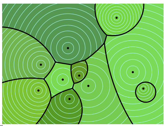
When we have Classes with Same Variance and Same Prior Probabilities, the decision boundary diagram becomes a Voronoi Diagram.

If we only have Same Variance but different Prior Probabilities, the decision boundary diagram becomes a Power Diagram.

A True Voronoi Diagram (Same Priors Probabilities)

---

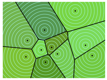
Voronoi Diagram : A Voronoi diagram divides a space into regions where each region corresponds to a "generator" point. Every location within a region is closer to its corresponding generator than to any other generator. Power Diagram: A power diagram, also known as a weighted Voronoi diagram, generalizes the concept of a Voronoi diagram by assigning a weight to each generator point. The distance metric is modified to account for these weights, leading to regions defined by the "power distance" rather than the standard Euclidean distance.

Maximum Likelihood Estimation