Anisotropic Gaussians

$X\sim \mathbf{N}(\mu ,\Sigma )$

The pdf of X is $\frac{1}{\sqrt{(2\pi {)}^2|\Sigma |}}\exp \left(-\frac{1}{2}(x-\mu {)}^T{\Sigma }^{-1}(x-\mu )\right)$

where, $|\Sigma |\text{is the determinant}$.

$\Sigma$ is the d x d PSD Covariance Matrix ${\Sigma }^{-1}$ is the d x d PSD Precision Matrix

For understanding the function easier, rewrite $f(x)=n(q(x))$ where $q(x)=(x-u{)}^T{\Sigma }^{-1}(x-u)$.

If we think carefully, we notice that $n(.)$ is a $fn:\mathbb{R}\to \mathbb{R}$, and $q(x)$ is a $fn:{\mathbb{R}}^d\to R$.

$q(x)$ is a quadratic function that we know. $q(x)$ is the quadratic form of the precision matrix ${\Sigma }^{-1}$ (a quadratic bowl with center at $\mu$). $n(.)$ is a monotonic, convex function: an exponential of the negation of the half of its argument. The graphs are shown below.

Left is q(x) : Quadratic Bowl. Right is the Probability Density Function. Notice how n(x) : exponential function transforms the graph.

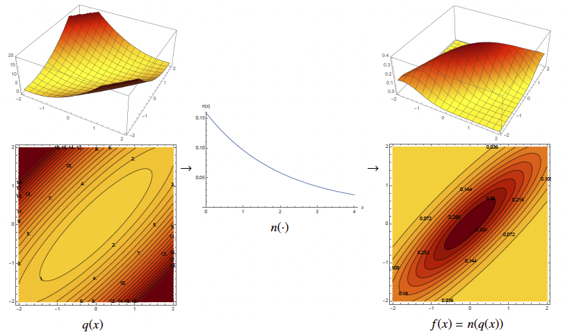
The two graphs have different isovalues, but the mapping doesn’t change its isosurfaces. Thus, minimization of q(x) is equivalent to the maximization of the probability distribution function.

Hint

Meaning of “Different isovalues but same isosurfaces”: This suggests that the contour levels (isovalues) of the function change, but the overall structure of the level sets (isosurfaces) remains the same. This typically happens when you apply a monotonic transformation to a function. In our case, this function is exponential function.

Summary

If you understand the isosurfaces of a quadratic function, then you understand the isosurfaces of a Gaussian, because they’re the same.

---

Remember from Visualizing Quadratic Form that the isocontours of $(x-u{)}^T{\Sigma }^{-1}(x-u)$ are determined by the eigenvalues and eigenvectors of ${\Sigma }^{1/2}$.

Side Notes

Remember from the induced norm theorem that, $q(x)$ is some sort of norm squared. In this case, having a precision matrix in the middle means that the norm is a sort of warped distance from x to mean $\mu$. Formally:

$$d(x,\mu )=\Vert {\Sigma }^{-1/2}x-{\Sigma }^{-1/2}\mu \Vert =\sqrt{(x-\mu {)}^T{\Sigma }^{-1}(x-\mu )}=\sqrt{q(x)}$$

Shewchuk

So we think of the precision matrix as a “metric tensor” which defines a metric, a sort of warped distance from x to the mean μ.