Agenda:
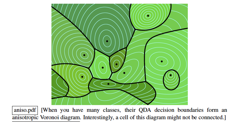
- Anisotropic QDA
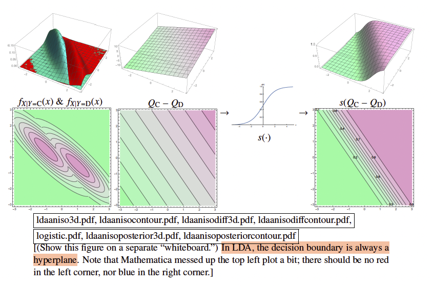
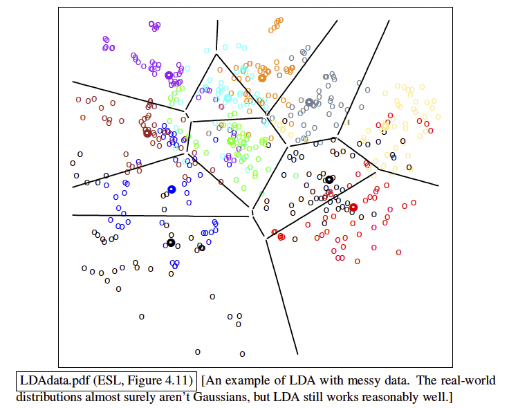
- Anisotropic LDA
- Isotropic QDA (already learned) (spherical)
- Isotropic LDA (spherical)
Maximum Likelihood Estimation for Anisotropic Gaussians
Given training points and classes , we need to find the best-fit Gaussians.
Let be the number of training points in class C.
Quadratic Discriminant Analysis (QDA)
- Covariance Matrix: The best estimate covariance matrix (conditional covariance of points in class C) , is:
- Discriminant Function:
- Decision Boundary:
- Posterior Probability (for two class):
- Visualization:

Linearly Discriminant Analysis (LDA)
- Covariance Matrix: For LDA, we want pool-covariance within-class matrix . **Note: This is a weighted sum with prior probabilities. **That means:
Note that is the same as prior probability of class C. And the rest of the terms is covariance of class C.
-
Discriminant Function:
-
Decision Boundary
-
Posterior Probability (for two class):
-
Visualization:
GDA vs LDA
For Two-classes Classification:
- LDA has
d+1parameters (w, ). - QDA has parameters.
- LDA is more likely to underfit (small number of parameters).
- QDA is more likely to overfit (the danger is much bigger wiith larger dimensions d) as the parameters grow with squared of the dimensions.
Cautions:
- that QDA or LDA on data doesn’t find the True Baye’s Classifier. In fact, it is not possible to get a true Baye’s Classifier since we do not know the true parameters / distribution of real world data. Most of the time, if not all the time, we use the estimated distributions from finite data. Moreover, real-world data might not fit the Gaussian perfectly.
- Changing Prior Probabilities or Loss Functions is the same as adding constants (actually
ln(constants)) to our discriminant functions. Thus, in a two-class classifiers, changing these values would be the same as simply changing isovalue. - Posterior Probability gives us some sort of confidence levels.
- Decision boundaries are drawn at different probability thresholds (e.g 10%, 50%, 90%) to indicate how confident we need to be before making a classification decision. 50% for 0-1 loss functions.
- Setting the decision boundary at probability
pis the same as setting asymmetric loss values for false positives and false negatives. (Similarly, the prior probability follows the same rule). - LDA can result in non-linear decision boundaries if we introduce new features or transformations.
Cite
LDA & QDA are the best method in practice for many applications. In the STATLOG project, either LDA or QDA were among the top three classifiers for 10 out of 22 datasets. But it’s not because all those datasets are Gaussian. LDA & QDA work well when the data can only support simple decision boundaries such as linear or quadratic, because Gaussian models provide stable estimates.